Setting up a lead scoring system in Excel can help you prioritize and manage your leads effectively. This guide will walk you through the process step-by-step, including examples and images to make it easy for you to follow along. Remember to make changes in the formulas as per your needs.

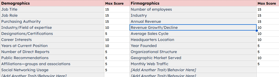
Step 1: Define Your Lead Scoring Criteria

First, you need to identify the criteria that are important for scoring your leads. Common criteria include:

• Company Size (Small, Medium, Large)
• Engagement Level (Low, Medium, High)
• Industry (Tech, Healthcare, Other)
• Location (US, Europe, Other)

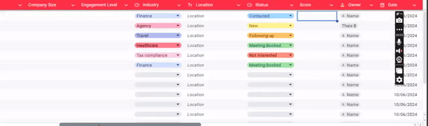
Step 2: Create Your Lead Data Table

Open Excel and create a new spreadsheet. Set up your table with the following columns:

• Lead Name
• Email
• Company Size
• Engagement Level
• Industry
• Location
• Lead Score

Step 3: Assign Points to Criteria

Decide on a point system for each criteria. For example:

• Company Size: Small (1 point), Medium (2 points), Large (3 points)
• Engagement Level: Low (1 point), Medium (2 points), High (3 points)
• Industry: Tech (3 points), Healthcare (2 points), Other (1 point)
• Location: US (3 points), Europe (2 points), Other (1 point)

Step 4: Use IF Statements for Each Criterion

In Excel, use IF statements to assign points based on each criterion.

1. Company Size:

In the column next to Company Size, enter the following formula to assign points:

=IF(C2="Small", 1, IF(C2="Medium", 2, IF(C2="Large", 3, 0)))

2. Engagement Level:

In the column next to Engagement Level, enter the following formula:

=IF(D2="Low", 1, IF(D2="Medium", 2, IF(D2="High", 3, 0)))

3. Industry:

In the column next to Industry, enter the following formula:

=IF(E2="Tech", 3, IF(E2="Healthcare", 2, 1))

4. Location:

In the column next to Location, enter the following formula:

=IF(F2="US", 3, IF(F2="Europe", 2, 1))

Step 5: Combine the Points into a Total Score

Sum up the points from each criterion to get a total lead score. In the Lead Score column, use the following formula:

=IF(C2="Small", 1, IF(C2="Medium", 2, IF(C2="Large", 3, 0))) +
IF(D2="Low", 1, IF(D2="Medium", 2, IF(D2="High", 3, 0))) +
IF(E2="Tech", 3, IF(E2="Healthcare", 2, 1)) +
IF(F2="US", 3, IF(F2="Europe", 2, 1))

Step 6: Apply the Formula to All Rows

Click and drag the fill handle (a small square at the bottom-right corner of the selected cell) down the column to apply the formula to all rows.

Example:

Step 7: Format Your Table

For better readability, format your table by adding borders, colors, and headers. Use conditional formatting to highlight high-scoring leads.

Step 8: Analyze and Use Your Lead Scores

Sort your table by the Lead Score column to prioritize your leads. Focus your efforts on the highest-scoring leads to maximize your chances of conversion.

Conclusion

Setting up a lead scoring system in Excel is a cost-effective way to manage and prioritize your leads. By following these steps and using the provided formulas (making the required adjustments for your needs), you can create a system that helps you focus on the most promising leads, ultimately improving your sales process and conversion rates.